Green’s Theorem
$$
$$
Another test for conservativeness
Given a differentiable function \(f\colon \mathbb{R}^2 \to \mathbb{R}\), its gradient is a conservative vector field \[\mathbf{F}(x,y) = \left\langle P(x,y), Q(x,y)\right\rangle = \mathbf{\nabla}f(x,y) = \left\langle f_x(x,y),f_y(x,y)\right\rangle\]
According to Clairaut’s Theorem, if \(f\) has continuous second partial derivatives, then the mixed second partial derivatives \(f_{xy}\) and \(f_{yx}\) are equal.
Since for a conservative vector field \(\mathbf{F} = \left\langle P,Q\right\rangle\), the components are \(P = f_x\) and \(Q = f_y\), the second partial derivatives of \(f\) are the first partial derivatives of \(P\) and \(Q\), and the mixed second partial derivatives of \(f\) are
\[\begin{aligned} f_{xy} &= P_y\\ f_{yx} &= Q_x \end{aligned}\]In other words, if we have a vector field \(\mathbf{F} = \left\langle P, Q\right\rangle\) such that both \(P\) and \(Q\) have continuous partial derivatives, and \(P_y \neq Q_x\), the field \(\mathbf{F}\) cannot be conservative! That gives us a new easier way to detect non-conservative vector fields without having to attempt to find a potential function!
Try it yourself
Some questions
There are some obvious questions we can ask about this:
What’s actually going on? What does the difference between \(P_y\) and \(Q_x\) have to do with conservativeness of the vector field?
Does it work the other way? Can we say that if \(P_y(x,y) = Q_x(x,y)\) then the vector field is conservative?
Can we extend this to 3 variables?
Let’s first graph the two examples of non-conservative vector fields, maybe it will give us some idea of what is going on:
The field \(\mathbf{F}(x,y) = \left\langle -y, x\right\rangle\):
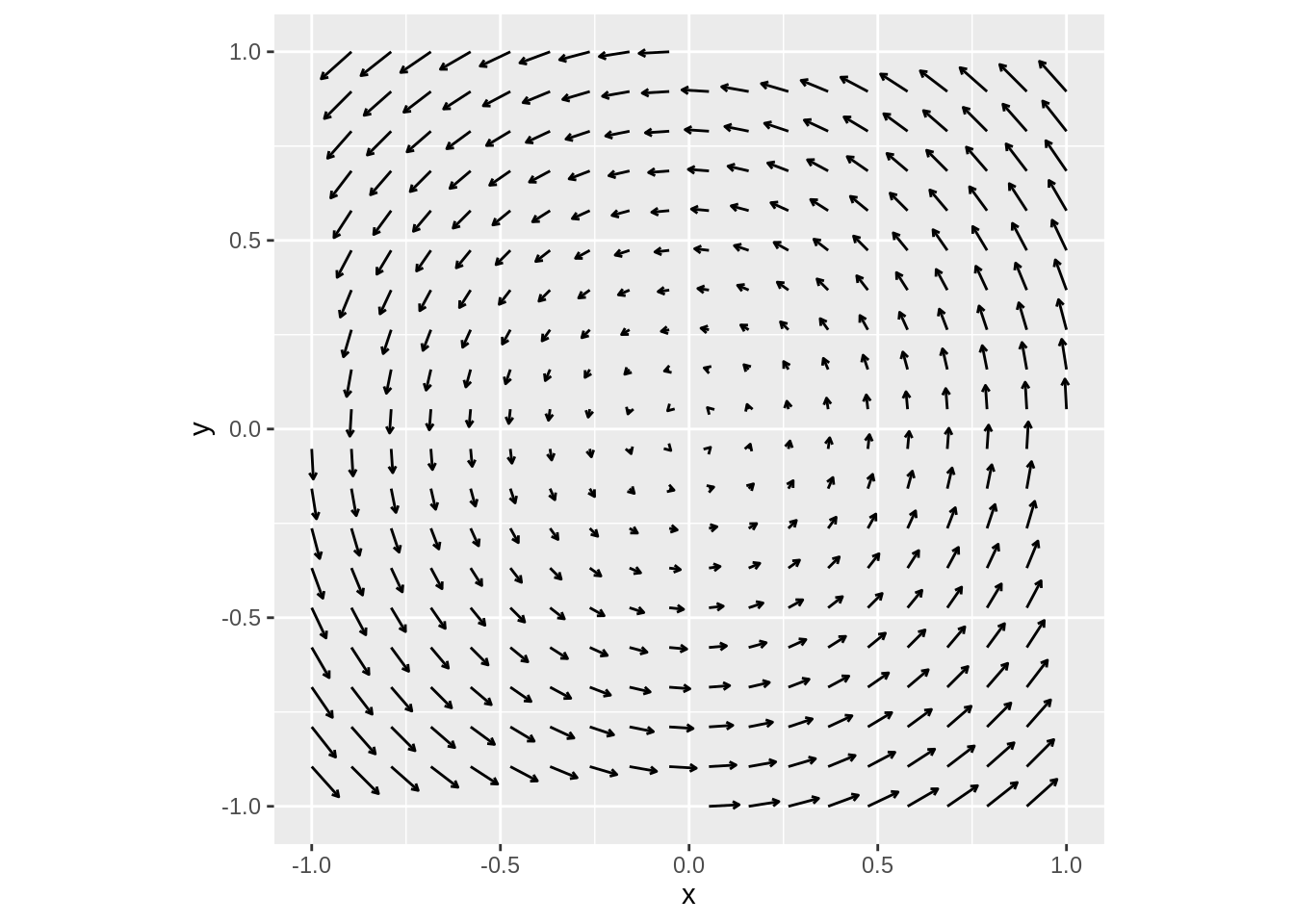
We can see clearly that this is not a conservative vector field: any integral over a circle centered at \((0,0)\) is going to be positive! This field seems to represent some sort of rotation around the origin.
The field \(\mathbf{F}(x,y) = \left\langle e^x\cos y, e^x\sin y\right\rangle\):
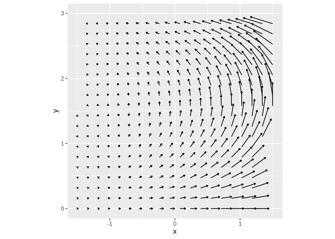
Again, we can see why this is non-conservative: while most arrows point generally upwards, the arrows on the right are much longer than the arrows on the left. If you insert any object into this force field somewhere near the center of the plot, the upward forces on the right side of the object will be much bigger than the upward forces on the left side of the object, causing the object to rotate counter-clockwise. An integral over any circle with center near the center of the plot window will be positive.
We want to better understand what does the equality of the partial derivatives of the field components have to do with conservativeness. Since derivatives are “local” properties, it may help to look at things at a really tiny scale. Let’s calculate a line integral of a vector field over a very very tiny rectangle centered at \((x_0,y_0)\), with sides of length \(dx\) and \(dy\). We will label the four sides of the rectangle as \(S_1\), \(S_2\), \(S_3\) and \(S_4\):

Then the integral of \(\mathbf{F}\) over the rectangle can be split into the sum of the integrals over the four sides:
\[ \int_{S_1} \mathbf{F}(x,y)\cdot \mathbf{dr} + \int_{S_2} \mathbf{F}(x,y)\cdot \mathbf{dr} + \int_{S_3} \mathbf{F}(x,y)\cdot \mathbf{dr} + \int_{S_4} \mathbf{F}(x,y)\cdot \mathbf{dr} \]
Reversing the direction of the integrals over \(S_3\) and \(S_4\) will give us
\[ \int_{S_1} \mathbf{F}(x,y)\cdot \mathbf{dr} + \int_{S_2} \mathbf{F}(x,y)\cdot \mathbf{dr} - \int_{-S_3} \mathbf{F}(x,y)\cdot \mathbf{dr} - \int_{-S_4} \mathbf{F}(x,y)\cdot \mathbf{dr} \]
Let’s approximate the four integrals:
We can parametrize the \(S_1\) curve as \(x = x_0 + t\), \(y = y_0 - \frac{dy}{2}\) for \(-\frac{dx}{2} \le t \le \frac{dx}{2}\).
Then \(dx = dt\) and \(dy = 0\), and so \[\int_{S_1} \mathbf{F}(x,y)\cdot\mathbf{dr} = \int_{-\frac{dx}{2}}^{\frac{dx}{2}} P\left(x_0 + t, y_0 - \frac{dy}{2}\right)\;dt\]If \(dx\) is very small, the last integral is approximately equal to \[P\left(x_0, y_0 - \frac{dy}{2}\right)\;dx\]
We can parametrize the \(-S_3\) curve as \(x = x_0 + t\), \(y = y_0 + \frac{dy}{2}\) for \(-\frac{dx}{2} \le t \le \frac{dx}{2}\).
Then \(dx = dt\) and \(dy = 0\), and so \[\int_{-S_3} \mathbf{F}(x,y)\cdot\mathbf{dr} = \int_{-\frac{dx}{2}}^{\frac{dx}{2}} P\left(x_0 + t, y_0 + \frac{dy}{2}\right)\;dt\]If \(dx\) is very small, the last integral is approximately equal to \[P\left(x_0, y_0 + \frac{dy}{2}\right)\;dx\]
We can parametrize the \(S_2\) curve as \(x = x_0 + \frac{dx}{2}\), \(y = y_0 + t\) for \(-\frac{dy}{2} \le t \le \frac{dy}{2}\).
Then \(dx = 0\) and \(dy = dt\), and so \[\int_{S_2} \mathbf{F}(x,y)\cdot\mathbf{dr} = \int_{-\frac{dy}{2}}^{\frac{dy}{2}} Q\left(x_0 + \frac{dx}{2}, y_0 + t\right)\;dt\]If \(dy\) is very small, the last integral is approximately equal to \[Q\left(x_0 + \frac{dy}{2}, y_0\right)\;dy\]
We can parametrize the \(-S_4\) curve as \(x = x_0 - \frac{dx}{2}\), \(y = y_0 + t\) for \(-\frac{dy}{2} \le t \le \frac{dy}{2}\).
Then \(dx = 0\) and \(dy = dt\), and so \[\int_{S_2} \mathbf{F}(x,y)\cdot\mathbf{dr} = \int_{-\frac{dy}{2}}^{\frac{dy}{2}} Q\left(x_0 - \frac{dx}{2}, y_0 + t\right)\;dt\]If \(dy\) is very small, the last integral is approximately equal to \[Q\left(x_0 - \frac{dy}{2}, y_0\right)\;dy\]
Looking at the two horizontal sides: if \(dx\) is very small,
\[\begin{aligned} \int_{S_1} \mathbf{F}(x,y)\cdot \mathbf{dr} - \int_{-S_3} \mathbf{F}(x,y)\cdot \mathbf{dr} &\approx P\left(x_0, y_0 - \frac{dy}{2}\right)\;dx - P\left(x_0, y_0 + \frac{dy}{2}\right)\;dx \\ &= \left(P\left(x_0, y_0 - \frac{dy}{2}\right) - P\left(x_0, y_0 + \frac{dy}{2}\right)\right)\;dx \\ &= \left(\frac{P\left(x_0, y_0 - \frac{dy}{2}\right) - P\left(x_0, y_0 + \frac{dy}{2}\right)}{dy}\right)\;dx\;dy \end{aligned}\]When \(dy\) is very small, \[\frac{P\left(x_0, y_0 - \frac{dy}{2}\right) - P\left(x_0, y_0 + \frac{dy}{2}\right)}{dy} \approx -P_y(x_0, y_0)\]
If both \(dx\) and \(dy\) are very small, then \[\int_{S_1} \mathbf{F}(x,y)\cdot \mathbf{dr} - \int_{-S_3} \mathbf{F}(x,y)\cdot \mathbf{dr} \approx -P_y(x_0, y_0)\;dx\;dy\]
Let’s now look at the two vertical sides: if \(dy\) is very small,
\[\begin{aligned} \int_{S_2} \mathbf{F}(x,y)\cdot \mathbf{dr} - \int_{-S_4} \mathbf{F}(x,y)\cdot \mathbf{dr} &\approx Q\left(x_0 + \frac{dx}{2}, y_0\right)\;dy - Q\left(x_0 + \frac{dx}{2}\right)\;dy \\ &= \left(Q\left(x_0 + \frac{dx}{2}, y_0\right) - Q\left(x_0 - \frac{dx}{2}, y_0\right)\right)\;dy \\ &= \left(\frac{Q\left(x_0 + \frac{dx}{2}, y_0\right) - Q\left(x_0 - \frac{dx}{2}, y_0\right)}{dx}\right)\;dx\;dy \end{aligned}\]When \(dx\) is very small, \[\frac{Q\left(x_0 + \frac{dx}{2}, y_0\right) - Q\left(x_0 - \frac{dx}{2}\right)}{dx} \approx Q_x(x_0, y_0)\]
If both \(dx\) and \(dy\) are very small, then \[\int_{S_2} \mathbf{F}(x,y)\cdot \mathbf{dr} - \int_{-S_4} \mathbf{F}(x,y)\cdot \mathbf{dr} \approx Q_x(x_0, y_0)\;dx\;dy\]
Putting all this together: when both \(dx\) and \(dy\) are very small, then the integral of \(\mathbf{F}(x,y)\) over the boundary of the small rectangle centered at \((x_0, y_0)\) with sides \(dx\) and \(dy\) is approximately equal to \[\left(Q_x(x_0, y_0) - P_y(x_0, y_0)\right)\;dx\;dy\] This approximation gets better the smaller \(dx\) and \(dy\) are1.
1 This argument can be actually made precise, without the need to refer to approximations, by using the Mean Value Theorem for derivatives and the Mean Value Theorem for definite integrals. It makes the whole derivation much more complicated, though.
Simple Curves and Circulation
Green’s Theorem
We saw that the quantity \[\left(Q_x(x,y) - P_y(x,y)\right)\;dx\;dy\] can be interpreted as a “local circulation” over an infinitesimal rectangle centered at \((x,y)\) with sides \(dx\) and \(dy\). We also was that circulation is “additive” in the sense that circulation over two simple curves that are adjacent to each other can be added. Intuitively this leads one to think that perhaps “summing” all local circulations at all interior points of a simple curve should give us a number that is equal to the circulation over the curve itself. Formally, this is expressed as the Green’s Theorem2:
2 The form of Green’s Theorem presented here is known as the Circulation form or Tangential form. There is also a form known as Flux form or Normal form. We are not covering it in this class, but you can find it in your textbook.
Suppose \(G\) is a region in a plane whose boundary \(\partial G\) is a piecewise smooth simple closed curve. Let \(\mathbf{F}(x,y) = \left\langle P(x,y), Q(x,y)\right\rangle\) be a vector field defined on \(G\) whose components have continuous partial derivatives on \(G\). Then \[\oint_{\partial G} \mathbf{F}(x,y)\cdot\mathbf{dr} = \iint_G \left(Q_x(x,y) - P_y(x,y)\right)\;dA\]
Above we gave an intuitive justification for the Green’s Theorem. The formal proof is beyond the scope of this class.
Note that this theorem is really a two-dimensional form of the Fundamental Theorem of Calculus. It says that an integral of some specific type of derivative of a vector field \(\mathbf{F}\) over a region \(G\) is equal to the integral of the vector field itself over the boundary of the region \(G\).
In the one-dimensional case, the “vector field” is just a real function of one variable, the “region” is just an interval, and its boundary consists of just two points.
Applications of Green’s Theorem
One more important consequence of Green’s Theorem is that the answer to our question 2 above is affirmative: If \(\mathbf{F} = \left\langle P(x,y), Q(x,y)\right\rangle\) is a vector field whose components have continuous partial derivatives, then \(\mathbf{F}\) is conservative if and only if \(Q_x(x,y) = P_y(x,y)\).