Local extrema and the second derivative test.
$$
$$
First derivatives and critical points
Suppose \(f\) is a differentiable function at a point \(A(a,b)\). It means that locally, the graph of the function looks like a plane with equation
\[z = f(a,b) + f_x(a,b)(x-a) + f_y(a,b)(y-b)\]
The normal vector of the plane is \(\left\langle -f_x(a,b), -f_y(a,b), 1\right\rangle\). The gradient vector \(\mathbf{\nabla} f(a,b) = \left\langle f_x(a,b), f_y(a,b)\right\rangle\) points in the direction in which \(f\) increases the fastest. And the directional derivative in the direction of the gradient vector at \((a,b)\) is equal to the magnitude of the gradient vector. If the magnitude of the gradient is positive, the function \(f\) is increasing in the direction of the gradient, and decreasing in the opposite direction.
Now suppose that the point \(A\) is the point of local maxima or minima of \(f\). That means the function cannot be increasing (if it is the maximum) or decreasing (if it is the minimum) in any direction, and the tangent plane cannot be slanted. It must be horizontal, with normal vector parallel to \(\mathbf{k}\).
From this we can conclude that if a function is differentiable at a point of local maxima or minima, the gradient vector at that point must be the zero vector.
This is very similar to the one-variable situation: If \(f'(a)\) exists at a point \(a\) that is a point of local maxima or minima, it must be 0.
Note that just like in the one-variable case, the converse is not true: It is possible to find points where the function is differentiable and the gradient is the zero vector, but the function does not have a local maximum or minimum at the point. We will see examples of that.
Other way this is often formulated is by saying that for a function differentiable at \(A\), zero gradient vector is necessary but not sufficient condition for the existence of local maximum or minimum at the point.
Just like in the single variable case, the usefulness of this is based on the contrapositive:
If the gradient vector of a differentiable function at \(A\) is not zero, then the function cannot have a local maximum or local minimum at \(A\).
The way we use this to find local maxima and minima is by first finding the points where a differentiable function has zero gradient vector (called critical points), and then further testing those points.
Examples of finding critical points
Second derivatives
One way we can sometimes find out what happens at critical points is by using the second derivative test.
In the single variable case, the second derivative test is very simple: if \(a\) is a point such that \(f'(a) = 0\), and \(f''(a) > 0\), then \(f\) is concave up at \(a\), and therefore must have a local minimum at \(a\). Similarly, if \(f''(a) < 0\), then \(f\) is concave down at \(a\), and the function has a local maximum at \(a\).
The situation is more complicated in two variables.
Quadratic functions
Let’s look at several examples of quadratic functions:
- \(f(x,y) = x^2 + xy + y^2\)
- \(f(x,y) = x^2 - xy + y^2\)
- \(f(x,y) = x^2 + 3xy + y^2\)
All of these functions have a critical point at \((0,0)\). Let’s look at traces of these functions through the origin, in the direction of a unit vector \(\mathbf{u}\): define a single variable function
\[g(t) = f(0 + u_1 t, 0 + u_2 t)\]
Almost all such functions are a quadratic functions (for the third function, there are 8 directions in which we get a constant zero function), so the graphs are parabolas. Some of them may be concave up, some may be concave down.
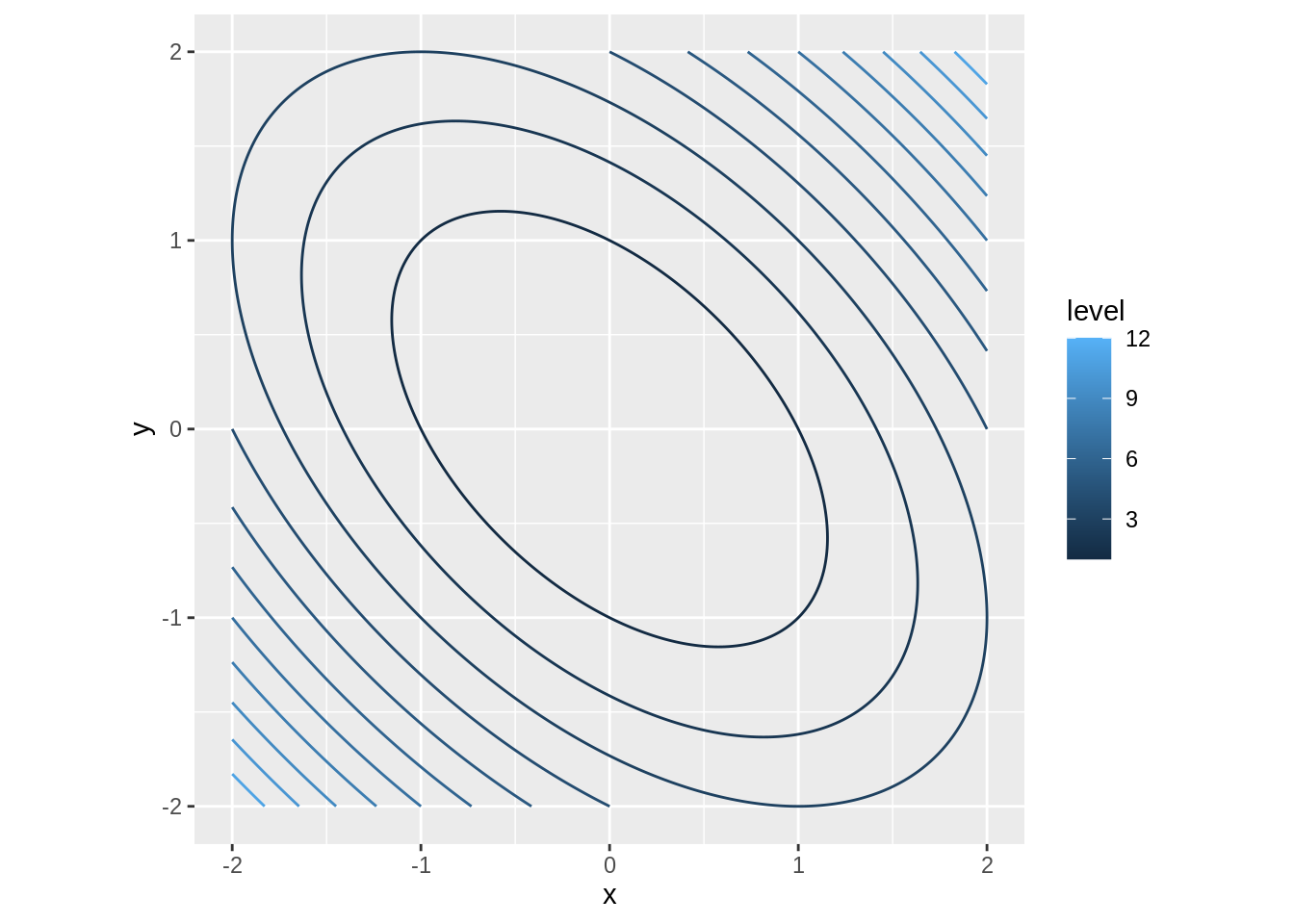
First function: \(f(x,y) = x^2 + xy + y^2\)
Here is the contour plot of the function:
Here is a video that shows an animation of three plots:
- The contour plot of the function together with the line \(\mathbf{r}(t) = \left\langle 0 + u_1 t, 0 + u_2 t\right\rangle\) as the vector \(\mathbf{u}\) spins around a full circle.
- The plot of the corresponding single variable function \(g\).
- The surface plot of \(f\), with the trace showing the plot of \(g\) embedded in the surface.
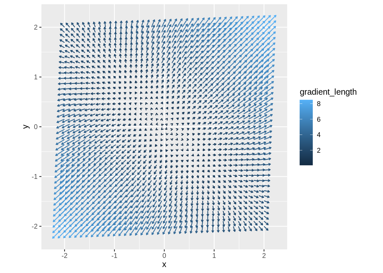
From all these plots we can see that there is a minimum at the point \((0,0)\). For completeness, here is the gradient plot of the function \(f\):
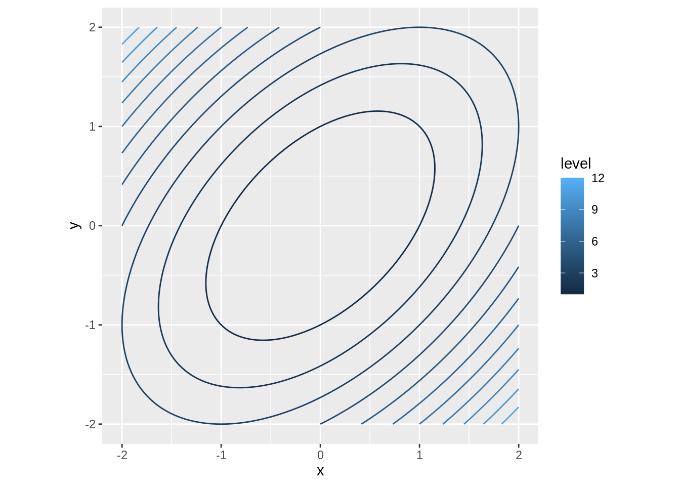
Second function: \(f(x,y) = x^2 - xy + y^2\)
Here is the contour plot of the function:
Here is the animation of the three plots, just like we did for the first function:
and here is the gradient plot:
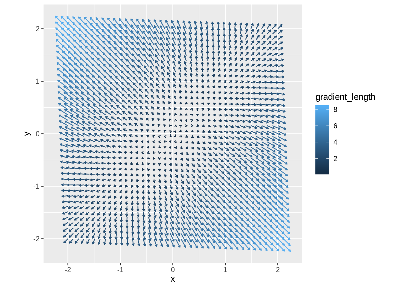
Again, all plots indicate a minimum at \((0,0)\).
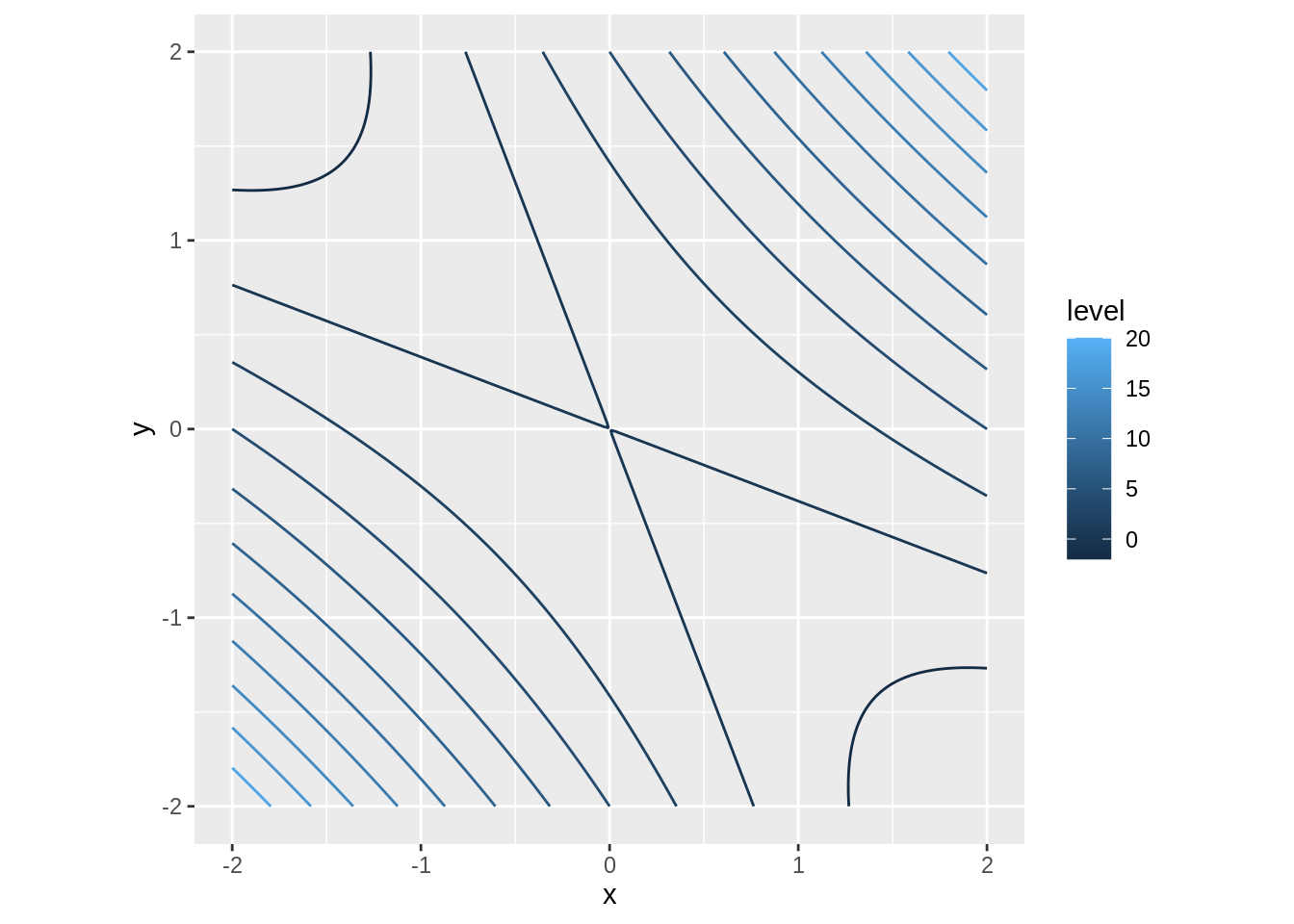
Third function: \(f(x,y) = x^2 + 3xy + y^2\)
This is a contour plot of \(f\):
Here is the animation of the three plots:
and here is the gradient plot:
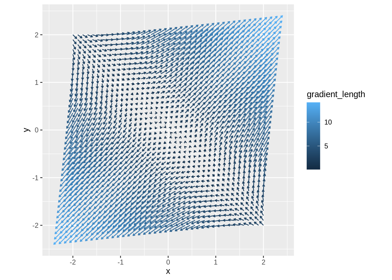
This time, the plots indicate a saddle point at \((0,0)\).
A general quadratic function
Let’s look at a general quadratic function in the form \(f(x,y) = ax^2 + bxy + cy^2\). This function has zero first derivatives at \((0,0)\) and \(f(0,0) = 0\).
Then for a unit vector \(\mathbf{u} = \left\langle u_1, u_2\right\rangle\), the corresponding function \(g\) is
\[g(t) = f(0 + u_1 t, 0 + u_2 t) = a(u_1 t)^2 + b u_1 u_2 t^2 + c (u_2 t)^2 = (a u_1^2 + b u_1 u_2 + c u_2^2) t^2\]
This is either a quadratic function or a constant zero function. If it is a quadratic function, its graph will be a parabola, that is concave up when \(a u_1^2 + b u_1 u_2 + c u_2^2 > 0\) and concave down when \(a u_1^2 + b u_1 u_2 + c u_2^2 < 0\).
If for all unit vectors \(\mathbf{u}\) the coefficient \(a u_1^2 + b u_1 u_2 + c u_2^2\) is positive, then \(f\) has a minimum at \((0,0)\).
If for all unit vectors \(\mathbf{u}\) the coefficient \(a u_1^2 + b u_1 u_2 + c u_2^2\) is negative, then \(f\) has a maximum at \((0,0)\).
If for some unit vectors \(\mathbf{u}\) the coefficient \(a u_1^2 + b u_1 u_2 + c u_2^2\) positive and for some it is negative, then \(f\) has a saddle point at \((0,0)\).
Finally, if there are are exactly two (parallel) unit vectors \(\mathbf{u}\) such that \(a u_1^2 + b u_1 u_2 + c u_2^2 = 0\) and \(a u_1^2 + b u_1 u_2 + c u_2^2\) is positive in all other directions (or negative in all other directions), then there is a whole line of maxima (or minima) passing through the origin:
To distinguish between these cases, we want to know how many solutions \((u_1, u_2)\) such that \(\mathbf{u} = \left\langle u_1, u_2\right\rangle\) is a unit vector does the equation \(a u_1^2 + b u_1 u_2 + c u_2^2 = 0\) have. If it has no solutions, then the coefficient \(a u_1^2 + b u_1 u_2 + c u_2^2\) is either always positive or always negative. If the equation has a solution, the coefficient could possibly change sign.
To make this easier, let’s split it into two cases:
Case \(a = 0\): In that case we have a solution \(u_2 = 0\) and, since we need a unit vector, \(u_1 = \pm 1\). On the other hand, assuming \(u_2 \neq 0\), we can divide by \(u_2^2\) and get \[b \frac{u_1}{u_2} + c = 0\] and if \(b \neq 0\) we get \[\frac{u_1}{u_2} = -\frac{c}{b}.\] In that case we have another pair of solutions:
\[\mathbf{u} = \left\langle u_1, u_2\right\rangle = \frac{\pm 1}{\sqrt{b^2 + c^2}}\left\langle c, b\right\rangle\]
So if \(a = 0\), we have at least two (if \(b = 0\)), possibly four (if \(b \neq 0\)), unit vectors such that \(a u_1^2 + b u_1 u_2 + c u_2^2 = 0\).
Case \(a \neq 0\): In that case we cannot have a solution with \(u_2 = 0\), because the only two unit vectors with \(u_2 = 0\) are \(\v{\pm 1, 0\}\), and plugging these into \(a u_1^2 + b u_1 u_2 + c u_2^2\) will not give us 0.
That means we can divide by \(u_2^2\), getting \[a\left(\frac{u_1}{u_2}\right)^2 + b\frac{u_1}{u_2} + c = 0\] and substituting \(s = \frac{u_1}{u_2}\) we get the quadratic equation \(as^2 + bs + c = 0\).
This has no real solution if \(b^2 - 4ac < 0\), exactly one real solution \(s\) if \(b^2 - 4ac = 0\) and two distinct real solutions \(s_1\) and \(s_2\) if \(b^2 - 4ac > 0\).
For each value of \(s\) there are two unit vectors \(\mathbf{u} = \left\langle u_1, u_2\right\rangle\) such that \(\frac{u_1}{u_2} = s\).
Note that if \(a = 0\), then \(b^2 - 4ac = b^2\) which is positive if \(b\neq 0\) and 0 if \(b = 0\), so we can combine both cases together, getting the following:
Conclusion: If \(f(x,y) = ax^2 + bxy + cy^2\), \(\mathbf{u} = \left\langle u_1, u_2\right\rangle\) is a unit vector, and \(g(t) = f(0 + u_1 t, 0 + u_2 t)\), then:
If \(4ac - b^2 > 0\), than the graphs of the functions \(g\) are either all parabolas concave up or all parabolas concave down. In that case the function \(f\) has either a maximum or a minimum at \((0,0)\).
If \(4ac - b^2 = 0\), then there are exactly two directly opposite direction in which the function \(g\) is a constant 0, and in all the other directions, either all the graphs of \(g\) are parabolas concave down or all the graphs of \(g\) are parabolas concave up. In that case the function \(f\) has infinitely many maxima or minima, that form a line passing through the origin.
If \(4ac - b^2 < 0\) than there are four directions in which the \(g\) is a constant zero, and in some of the other directions, the graph of \(g\) is a parabola concave down, while in other directions the graph of \(g\) is a parabola concave up. In that case the function \(f\) has a saddle point at \((0,0)\).
Second derivative test
Let \(f:\mathbb{R}^2 \to \mathbb{R}\) be a function with a critical point \((x_0,y_0)\) such that \(f\) is at least twice continuously differentiable on some disk centered at \((x_0,y_0)\). According to the Taylor’s Theorem, if \((x,y)\) is close to \((x_0,y_0)\), \(f(x,y)\) can be approximated by
\[\begin{aligned} f(x,y) &= f(x_0,y_0) + f_x(x_0,y_0)(x - x_0) + f_y(x_0,y_0)(y - y_0)\\ &+ \frac{1}{2}\left(f_{xx}(x_0,y_0)(x - x_0)^2 + 2f_{xy}(x_0,y_0)(x-x_0)(y-y_0) + f_{yy}(x_0,y_0)(y-y_0)^2\right)\\ &+ E(x,y) \end{aligned}\]with the approximation error \(\left\lvert E(x,y) \right\rvert < C\left(\sqrt{(x-x_0)^2 + (y-y_0)^2}\right)^3\) for some positive constant \(C\).
Since \((x_0,y_0)\) is a critical point of \(f\), \(f_x(x_0,y_0) = f_y(x_0,y_0) = 0\), so the above becomes
\[ f(x_0,y_0) + \frac{1}{2}\left(f_{xx}(x_0,y_0)(x - x_0)^2 + 2f_{xy}(x_0,y_0)(x-x_0)(y-y_0) + f_{yy}(x_0,y_0)(y-y_0)^2\right) \]
and substituting \(a = f_{xx}(x_0,y_0)\), \(b = 2f_{xy}(x_0,y_0)\) and \(c = f_{yy}(x_0,y_0)\), we get
\[f(x,y) = f(x_0, y_0) + \frac{1}{2}\left({\color{red}a(x-x_0)^2 + b(x-x_0)(y-y_0) + c(y-y_0)^2}\right) + E(x,y)\]
The expression in the parentheses is a quadratic function of two variables, like the ones we discussed above, and
- has a minimum or maximum at \((x_0, y_0)\) if \(4ac - b^2 > 0\),
- is constant 0 on a line passing through \((x_0,y_0)\) if \(4ac - b^2 = 0\),
- has a saddle point at \((x_0,y_0)\) if \(4ac - b^2 < 0\).
In the case 1 or 3 happens, the approximation error will be too small to affect this behavior for \((x,y)\) close to \((x_0, y_0)\), and so the function \(f\) itself will have a maximum or minimum or saddle point, as indicated by \(4ac - b^2\), at \((x_0, y_0)\).
If 2 happens, however, the approximation error can change the horizontal line passing through \((x_0,y_0)\) in such a way that the point \((x_0, y_0)\) is no longer a maximum or a minimum. In that case it is impossible to tell whether \(f\) has a maximum or minimum or saddle point just by looking at second derivatives. Similarly, if \(a = b = c = 0\), that is all the second partial derivatives are zero, the behavior of \(f\) cannot be determined from the second partial derivatives alone.
Finally, if we plug back in for \(a\), \(b\) and \(c\),
\[\begin{aligned} 4ac - b^2 &= 4f_{xx}(x_0, y_0)f_{yy}(x_0, y_0) - \left(2f_{xy}(x_0, y_0)\right)^2\\ &= 4\left(f_{xx}(x_0,y_0)f_{yy}(x_0,y_0) - \left(f_{xy}(x_0,y_0)\right)^2\right) \end{aligned}\]Since we are only interested in the sign of this expression, we can drop the factor \(4\) and just look at
\[f_{xx}(x_0,y_0)f_{yy}(x_0,y_0) - \left(f_{xy}(x_0,y_0)\right)^2\]
Conclusion
The Second Derivative Test: Let \(f:\mathbb{R}^2 \to \mathbb{R}\) be differentiable at \((x_0, y_0)\), with \((x_0, y_0)\) being a critical point of \(f\), such that the second partial derivatives of \(f\) are continuous on some disk centered at \((x_0, y_0)\).
Define the discriminant \(D = f_{xx}(x_0,y_0)f_{yy}(x_0, y_0) - \left(f_{xy}(x_0,y_0)\right)^2\)
- If \(D > 0\), then \(f\) has a local maximum (if \(f_{xx}\) and \(f_{yy}\) are both negative) or local minimum (if \(f_{xx}\) and \(f_{yy}\) are both positive) at \((x_0, y_0)\).
- If \(D < 0\) than \(f\) has a saddle point at \((x_0, y_0)\).
- If \(D = 0\), the second derivative test is inconclusive, and further investigation is needed to determine what is happening at \((x_0, y_0)\).
Note: Under the assumption of the test, \(f_{xy}(x_0, y_0) = f_{yx}(x_0, y_0)\). We can also write the discriminant as
\[D = f_{xx}(x_0, y_0) f_{yy}(x_0, y_0) - f_{xy}(x_0, y_0)f_{yx}(x_0, y_0)\]
however, the difference is purely cosmetic.
We can also write the discriminant as a determinant:
\[D = \left\lvert \begin{matrix} f_{xx}(x_0, y_0) & f_{xy}(x_0, y_0)\\ f_{yx}(x_0, y_0) & f_{yy}(x_0, y_0) \end{matrix} \right\rvert\]
This is called the Hessian determinant of the function \(f\) at \((x_0, y_0)\). The matrix
\[\begin{pmatrix} f_{xx}(x_0, y_0) & f_{xy}(x_0, y_0)\\ f_{yx}(x_0, y_0) & f_{yy}(x_0, y_0) \end{pmatrix}\]is called the Hessian matrix (or simply Hessian) of \(f\) at \((x_0, y_0)\).
Examples
Example of a function with \(f_{xx}(0,0) = 2.1\), \(f_{yy}(0,0) = 1.2\) and \(f_{xy}(0,0) = .6\):
Example of a function with \(f_{xx}(0,0) = 2.1\), \(f_{yy}(0,0) = .7\) and \(f_{xy}(0,0) = 3.3\):
Example of a function with \(f_{xx}(0,0) = 2.1\), \(f_{yy}(0,0) = .6\) and \(f_{xy}(0,0) = -1.2\):
Example of a function with \(f_{xx}(0,0) = 2.4\), \(f_{yy}(0,0) = .6\) and \(f_{xy}(0,0) = 1.2\). Here the second derivative test is inconclusive: